Raster Suitability Model

Introduction and Goals: 

The final lab of this course will be to create a mine suitability model for Trempealeau County, Wisconsin. As has been previously stated in the labs, Trempealeau County, located in western Wisconsin located in a region very popular for frac sand mining. We will be looking specifically at the lower half of the county. This is primarily done so the geoprocessing processing takes a shorter amount of time.

Two models will be used: one to show where sand mining is suitable and the other to show where sand mining is risky. This index determines where it would be best to develop frac sand mines in Trempealeau County (figure 1). The goal is to create a final map which depicts the best locations for sand mining with minimal impacts to the environment and humans.

Figure 1. Study area for raster suitability model, located in Trempealeau County, Wisconsin.

Objectives:

Suitability for mining

Generate a spatial data layer to meet the criteria for:
1. Geology
2. Land Cover (suitable and non-suitable)
3. Proximity to Rail Terminal
4. Slope
5. Water-table depth

6. Then combine the criteria to develop a suitability index model

Risk for mining

Generate a spatial data layer to measure impacts to: 
1. Streams
2. Prime farmland
3. Residential and populated areas
4. Schools
5. Wildlife areas

6. Then combine the factors into a risk model
7. Examine the results in proximity to prime recreational areas

Methods and Results:

The work flow seen below (figure 2) developed the first suitability model. Some of the input feature classes that were originally vector needed to be changed from a feature to raster, this was done using the 'Feature to Raster' tool. The 'Euclidean Distance' tool created a distance to closest source raster. This tool basically serves as a 'Buffer' tool within raster. The 'Reclassify' tool was then run to rank the distance of the nominal variable as being suitable, or not suitable for frac sand mine location. The raster calculator was used to add the reclassified feature classes, which resulted in a suitability index.

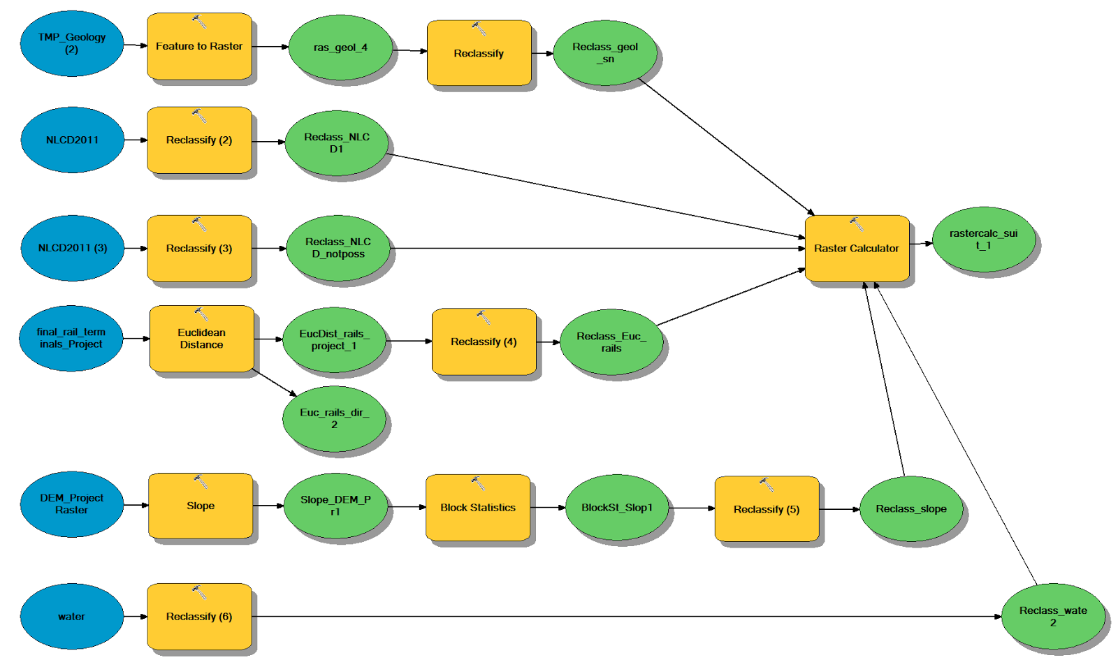Figure 2. Workflow for the suitability model. The final tool 'added up' the suitability of  geology (suitable), land use (suitable), land use (not suitable), proximity to railroads, slope (suitable), and depth to water table (suitable). The raster were reclassified manually using the below parameters (see below in figure 3) to develop a single impact map (see below in figure 4).

As stated above, reclassification is vital in order to make the suitability model accurate. Below illustrates the classification that was manually inputted (figure 3) to create the most appropriate suitability model. The higher the ranking, the more suitable the area is for a mine site. The ranks labeled '0' are not at all suitable for a mine site.

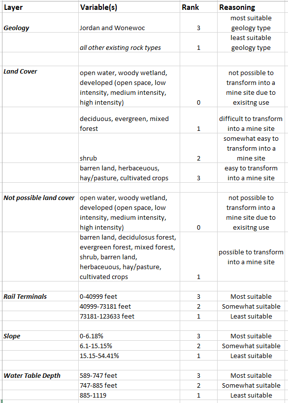Figure 3. Reclassification of rasters for suitability model including geology, land use (suitable), land use (not possible), proximity to railroads, and slope (suitable).

The individual maps that were created from the reclassification are seen below (figure 4). The green areas on the maps were manually ranked the highest in the reclassification tool. The center top map (figure 4) was calculated using the 'Raster Calculator' tool to 'add up' the rasters. 

Figure 4. Mine suitability model maps. These maps depict locations where the land is most utilized for its resources.  

A very similar workflow was used on the impact model. The feature classes in the model include streams, prime farmland, residential areas, schools, and wildlife areas. The workflow can be seen below (figure 5).

Figure 5. Workflow for the mine impact model. The final tool 'added up' the impacts of the variables (streams, schools, residential areas, wildlife areas, and prime farmland). The raster were reclassified manually (as seen below in figure 6) to develop a single impact map (see below in figure 7).

The specific reclassification ranks that were assigned to the features (figure 6). Unlike the suitability model, a high rank was given to features that are the most impactful to the environment and people.Below illustrates the classification that was manually inputted (figure 6) to create the most appropriate impact model. The distances are all ranked similarly because the closer the mine is to the feature (ie streams and prime farmland), the more impacted the feature is.

Figure 6. Reclassification of rasters for impact model.

Figure 7. The red regions depict the areas that are impacted by mining the most, whereas the green areas indicate the least impacted areas for mining. The top center map is the impact model which took into account the impact that mining has on streams, schools, residential areas, wildlife areas, and prime farmland.

An additional analysis piece that was used during the lab was a weighted impact model. This was done through Py Scripter to determine a weighted index model using features of the previous impact model, with specific weight on the residential area, thus making that specific feature more 'important'. A weight of '1.5' was used to emphasize residential areas. The script for the lab can be seen here. A comparative map was created to show the difference between the weighted and regular impact models (figure 8).

Figure 8. Comparative model of the weighted and normal impact models. Note that the residential areas (the large squares), are seen as being more impacted in the weighted impact model than the normal impact model.

Another added component that was included for this lab was using the viewshed tool. This tool takes an observation point and calculates the estimated area that can be seen from the observation point using a digital elevation model (DEM).

Figure 9. Viewshed model. The output map for the viewshed tool is seen below in figure 10.

Figure 10. Viewshed tool map. 

The final set in completing the overall suitability model was using the raster calculator tool to 'add up' the calculated impact and calculated suitability features. The workflow can be seen below (figure 11). Its related map is also below (figure 12)

Figure 11. Workflow for the suitability and impact model. This model integrated all of the models created in this lab including the impact and suitability index.

Figure 12. Final suitability and impact model. The map depicts the location where is it best to mine in Trempealeau County while minimizing disturbances (such as streams and residential areas) and maximizing resources (such as depth to water table and proximity to nearest rail terminal). 

Conclusion:

As frac sand mining will likely become more popular as demand for the sand increases, it is important to develop accurate and relevant suitability models. Without the proper use of this GIS technology, there could be many implications that could leave the environment, people, and mining resources in jeopardy. Not only that, but the specific mining company that would hypothetically use our suitability model could lose millions of dollars from developing a mine on unsuitable land.

Discussion:

One of the most challenging components of creating the suitability model was creating a logical ranking for the reclassification. It is very easy to develop a random numbering system, but to make the project more accurate, it is important to consider logical breaks when reclassifying rasters. This takes someone who has a relatively expansive knowledge of the subject and how it should be applied in the real world.

Through trial and error throughout this lab, it is apparent that it is very easy to 'sway' the data depending on how the rasters are reclassified, however, it is very important to take time and consider the implications of a miscalculated impact or suitability model.

I personally really enjoyed this lab because it is extremely relevant to the real world and used a large number of the tools that I have gained over my two formal GIS courses. It is labs like this that get me excited to be able to use GIS as a took to make important environmental decisions in the future.

Source: 

Bureau of Transportation Statistics. (n.d.). Rail terminals feature class. Retrieved December 6, 2015, from http://www.rita.dot.gov/bts/sites/rita.dot.gov.bts/files/subject_areas/geographic_information_services/index.html 

Land Records. (n.d.). Trempealeau County Land Records. Geodatabase. Retrieved December 6, 2015, from http://www.tremplocounty.com/landrecords/ 

United States Geological Survey, National Map Viewer. National Land Cover Database (NLCD) raster and DEM. (n.d). Retrieved December 6, 2015, from http://nationalmap.gov/viewer.html

Wisconsin Geological and Natural History Survey (GNHS). Water table contours. GIS data. (n.d). Retrieved December 6, 2015, from http://wgnhs.uwex.edu/map-data/gis-data/

Wisconsin Geological and Natural History Survey (WGNHS). B.A. Brown, 1988. Bedrock Geology of Wisconsin, West-Central Sheet, WGNHS Map 104. Digitizing by Beatriz Vidru Linhares, University of Wisconsin Eau Claire (UWEC). Retrieved from UWEC GIS resources.